Assignment 5

Histogram and barchart

worlds_fairs <- na.omit(readr::read_csv('https://raw.githubusercontent.com/rfordatascience/tidytuesday/master/data/2024/2024-08-13/worlds_fairs.csv'))

Rows: 70 Columns: 14
── Column specification ────────────────────────────────────────────────────────
Delimiter: ","
chr (6): name_of_exposition, country, city, category, theme, notables
dbl (8): start_month, start_year, end_month, end_year, visitors, cost, area,...

ℹ Use `spec()` to retrieve the full column specification for this data.
ℹ Specify the column types or set `show_col_types = FALSE` to quiet this message.

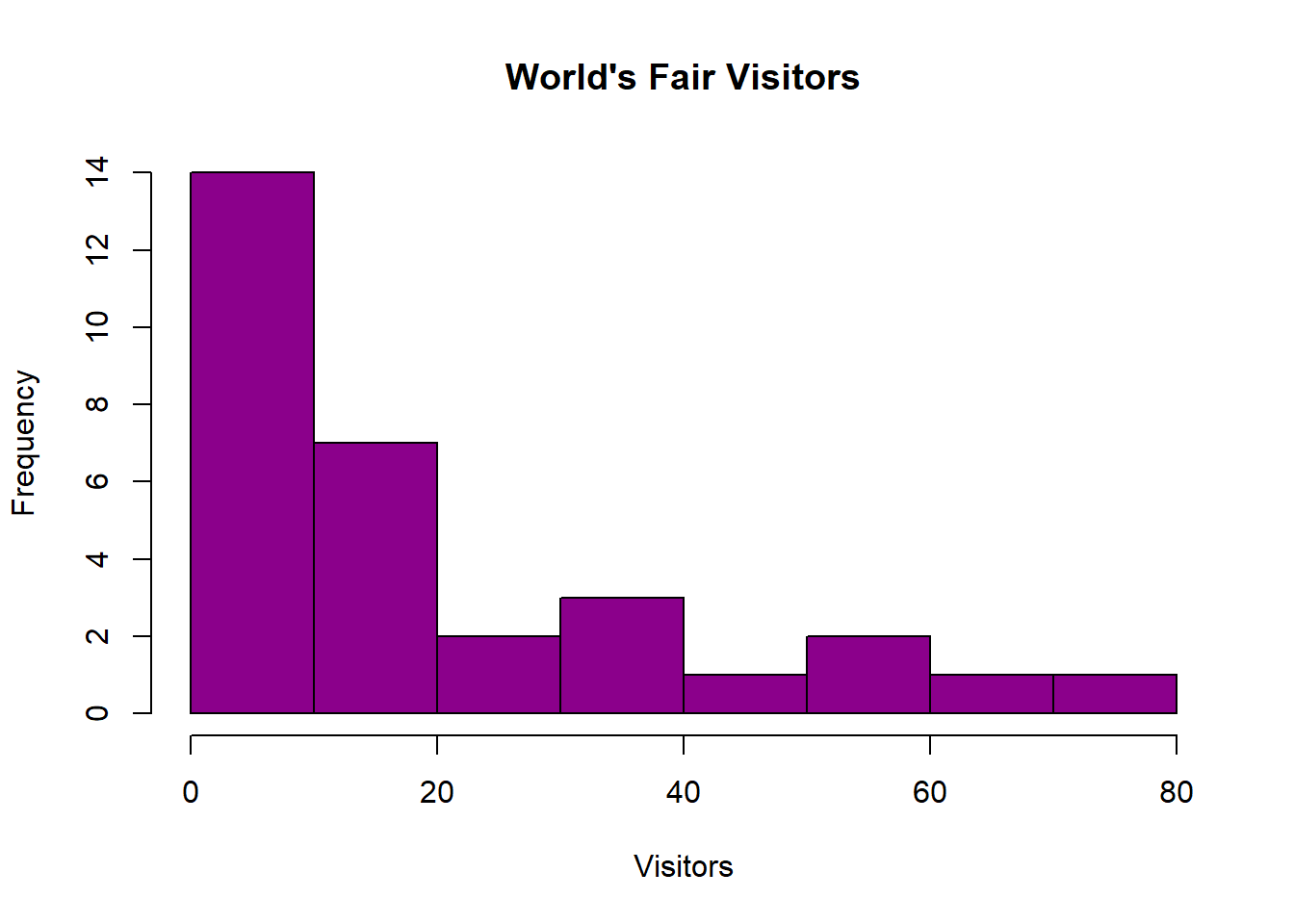
hist(worlds_fairs$visitors, xlab = "Visitors", main = "World's Fair Visitors", col = "magenta4")

text(
barplot(worlds_fairs$attending_countries,names.arg = worlds_fairs$start_year, col = "steelblue", ylim = c(0, max(worlds_fairs$attending_countries) * 1.2)),
  y = worlds_fairs$attending_countries + 1.5, labels = worlds_fairs$country, pos = 3, cex = .7, col = "black",srt=90, ylab = "Attending Countries", xlab = "Start Year", main = "World's Fair Attending Countries"
)

barplot(worlds_fairs$cost,names.arg=worlds_fairs$start_year, horiz = TRUE, col = "darkgreen",las=2,ylab = "Start Year", xlab = "Cost", main = "World's Fair Cost")

Piechart

slices <- table(worlds_fairs$category)
pct <- round(slices/sum(slices)*100)
lbls <- paste(rev(unique(worlds_fairs$category)), pct)
# add percents to labels
lbls <- paste(lbls,"%",sep="")
pie(slices,labels = lbls, col=rainbow(length(lbls)),
   main="Pie Chart of World's Fair Categories")

boxplot

boxplot(worlds_fairs$visitors,
main = "World's Fair Visitors",
xlab = "Visitors in millions",
ylab = "Fairs",
col = "orange",
border = "brown",
horizontal = TRUE,
notch = TRUE
)

Scatterplot

plot(worlds_fairs$start_year, worlds_fairs$visitors, pch=20, col="purple4", ylab = "Visitos in millions", xlab = "Year", main = "World's Fair Visitors by Year")
text(worlds_fairs$start_year, worlds_fairs$visitors, labels=worlds_fairs$name_of_exposition, cex= 0.6, pos=3)

ggplot scatterplot

library("ggplot2")
ggplot(worlds_fairs, aes(x = start_year, y = visitors)) +
    geom_point(aes(x = start_year, 
                   y = visitors, 
                   color = category),size = 2) +
  geom_text(aes(start_year,visitors,label=name_of_exposition),position = position_dodge(width=0.9),  size=2) +
  theme_minimal()+
  ggtitle("Year by Visitors") +
  xlab("Year") +
  ylab("Visitors in Millions")

File Types

#pdf(file = 'my_plot.pdf') PDF is a document format
#jpeg(file = 'my_plot.jpeg') compressable format for images on the internet
#tiff(file = 'my_plot.tiff') High quality image format
#svg(file = 'my_plot.svg')  scalable image format
#bmp(file = 'my_plot.bmp')  uncompressed raster format

#plot to export
# slices <- table(worlds_fairs$category)
# pct <- round(slices/sum(slices)*100)
# lbls <- paste(rev(unique(worlds_fairs$category)), pct)
# # add percents to labels
# lbls <- paste(lbls,"%",sep="")
# pie(slices,labels = lbls, col=rainbow(length(lbls)),
#    main="Pie Chart of World's Fair Categories")

#end export
#dev.off()

pdf

jpef

jpg tiff

svg

bmp