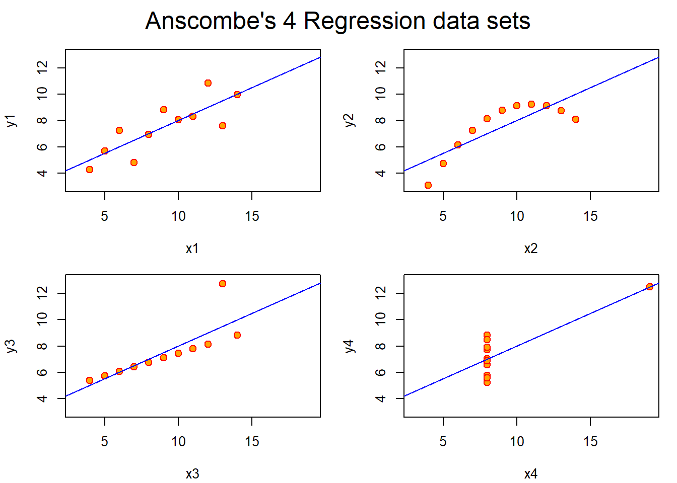
       x1             x2             x3             x4           y1
 Min.   : 4.0   Min.   : 4.0   Min.   : 4.0   Min.   : 8   Min.   : 4.260
 1st Qu.: 6.5   1st Qu.: 6.5   1st Qu.: 6.5   1st Qu.: 8   1st Qu.: 6.315
 Median : 9.0   Median : 9.0   Median : 9.0   Median : 8   Median : 7.580
 Mean   : 9.0   Mean   : 9.0   Mean   : 9.0   Mean   : 9   Mean   : 7.501
 3rd Qu.:11.5   3rd Qu.:11.5   3rd Qu.:11.5   3rd Qu.: 8   3rd Qu.: 8.570
 Max.   :14.0   Max.   :14.0   Max.   :14.0   Max.   :19   Max.   :10.840
       y2              y3              y4
 Min.   :3.100   Min.   : 5.39   Min.   : 5.250
 1st Qu.:6.695   1st Qu.: 6.25   1st Qu.: 6.170
 Median :8.140   Median : 7.11   Median : 7.040
 Mean   :7.501   Mean   : 7.50   Mean   : 7.501
 3rd Qu.:8.950   3rd Qu.: 7.98   3rd Qu.: 8.190
 Max.   :9.260   Max.   :12.74   Max.   :12.500
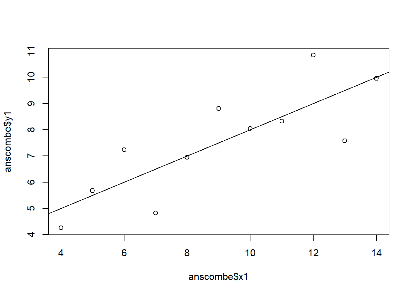
Call:
lm(formula = y1 ~ x1, data = anscombe)

Residuals:
     Min       1Q   Median       3Q      Max
-1.92127 -0.45577 -0.04136  0.70941  1.83882

Coefficients:
            Estimate Std. Error t value Pr(>|t|)
(Intercept)   3.0001     1.1247   2.667  0.02573 *
x1            0.5001     0.1179   4.241  0.00217 **
---
Signif. codes:  0 '***' 0.001 '**' 0.01 '*' 0.05 '.' 0.1 ' ' 1

Residual standard error: 1.237 on 9 degrees of freedom
Multiple R-squared:  0.6665,    Adjusted R-squared:  0.6295
F-statistic: 17.99 on 1 and 9 DF,  p-value: 0.00217
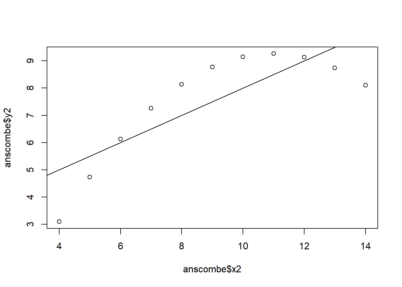
Call:
lm(formula = y2 ~ x2, data = anscombe)

Residuals:
    Min      1Q  Median      3Q     Max
-1.9009 -0.7609  0.1291  0.9491  1.2691

Coefficients:
            Estimate Std. Error t value Pr(>|t|)
(Intercept)    3.001      1.125   2.667  0.02576 *
x2             0.500      0.118   4.239  0.00218 **
---
Signif. codes:  0 '***' 0.001 '**' 0.01 '*' 0.05 '.' 0.1 ' ' 1

Residual standard error: 1.237 on 9 degrees of freedom
Multiple R-squared:  0.6662,    Adjusted R-squared:  0.6292
F-statistic: 17.97 on 1 and 9 DF,  p-value: 0.002179
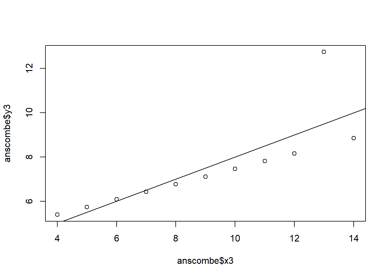
Call:
lm(formula = y3 ~ x3, data = anscombe)

Residuals:
    Min      1Q  Median      3Q     Max
-1.1586 -0.6146 -0.2303  0.1540  3.2411

Coefficients:
            Estimate Std. Error t value Pr(>|t|)
(Intercept)   3.0025     1.1245   2.670  0.02562 *
x3            0.4997     0.1179   4.239  0.00218 **
---
Signif. codes:  0 '***' 0.001 '**' 0.01 '*' 0.05 '.' 0.1 ' ' 1

Residual standard error: 1.236 on 9 degrees of freedom
Multiple R-squared:  0.6663,    Adjusted R-squared:  0.6292
F-statistic: 17.97 on 1 and 9 DF,  p-value: 0.002176
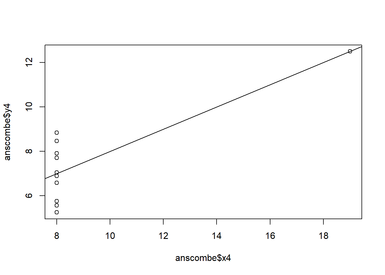
Call:
lm(formula = y4 ~ x4, data = anscombe)

Residuals:
   Min     1Q Median     3Q    Max
-1.751 -0.831  0.000  0.809  1.839

Coefficients:
            Estimate Std. Error t value Pr(>|t|)
(Intercept)   3.0017     1.1239   2.671  0.02559 *
x4            0.4999     0.1178   4.243  0.00216 **
---
Signif. codes:  0 '***' 0.001 '**' 0.01 '*' 0.05 '.' 0.1 ' ' 1

Residual standard error: 1.236 on 9 degrees of freedom
Multiple R-squared:  0.6667,    Adjusted R-squared:  0.6297
F-statistic:    18 on 1 and 9 DF,  p-value: 0.002165
Analysis of Variance Table

Response: y1
          Df Sum Sq Mean Sq F value  Pr(>F)
x1         1 27.510 27.5100   17.99 0.00217 **
Residuals  9 13.763  1.5292
---
Signif. codes:  0 '***' 0.001 '**' 0.01 '*' 0.05 '.' 0.1 ' ' 1
Analysis of Variance Table

Response: y2
          Df Sum Sq Mean Sq F value   Pr(>F)
x2         1 27.500 27.5000  17.966 0.002179 **
Residuals  9 13.776  1.5307
---
Signif. codes:  0 '***' 0.001 '**' 0.01 '*' 0.05 '.' 0.1 ' ' 1
Analysis of Variance Table

Response: y3
          Df Sum Sq Mean Sq F value   Pr(>F)
x3         1 27.470 27.4700  17.972 0.002176 **
Residuals  9 13.756  1.5285
---
Signif. codes:  0 '***' 0.001 '**' 0.01 '*' 0.05 '.' 0.1 ' ' 1
Analysis of Variance Table

Response: y4
          Df Sum Sq Mean Sq F value   Pr(>F)
x4         1 27.490 27.4900  18.003 0.002165 **
Residuals  9 13.742  1.5269
---
Signif. codes:  0 '***' 0.001 '**' 0.01 '*' 0.05 '.' 0.1 ' ' 1
                  lm1      lm2       lm3       lm4
(Intercept) 3.0000909 3.000909 3.0024545 3.0017273
x1          0.5000909 0.500000 0.4997273 0.4999091
$lm1
             Estimate Std. Error  t value    Pr(>|t|)
(Intercept) 3.0000909  1.1247468 2.667348 0.025734051
x1          0.5000909  0.1179055 4.241455 0.002169629

$lm2
            Estimate Std. Error  t value    Pr(>|t|)
(Intercept) 3.000909  1.1253024 2.666758 0.025758941
x2          0.500000  0.1179637 4.238590 0.002178816

$lm3
             Estimate Std. Error  t value    Pr(>|t|)
(Intercept) 3.0024545  1.1244812 2.670080 0.025619109
x3          0.4997273  0.1178777 4.239372 0.002176305

$lm4
             Estimate Std. Error  t value    Pr(>|t|)
(Intercept) 3.0017273  1.1239211 2.670763 0.025590425
x4          0.4999091  0.1178189 4.243028 0.002164602