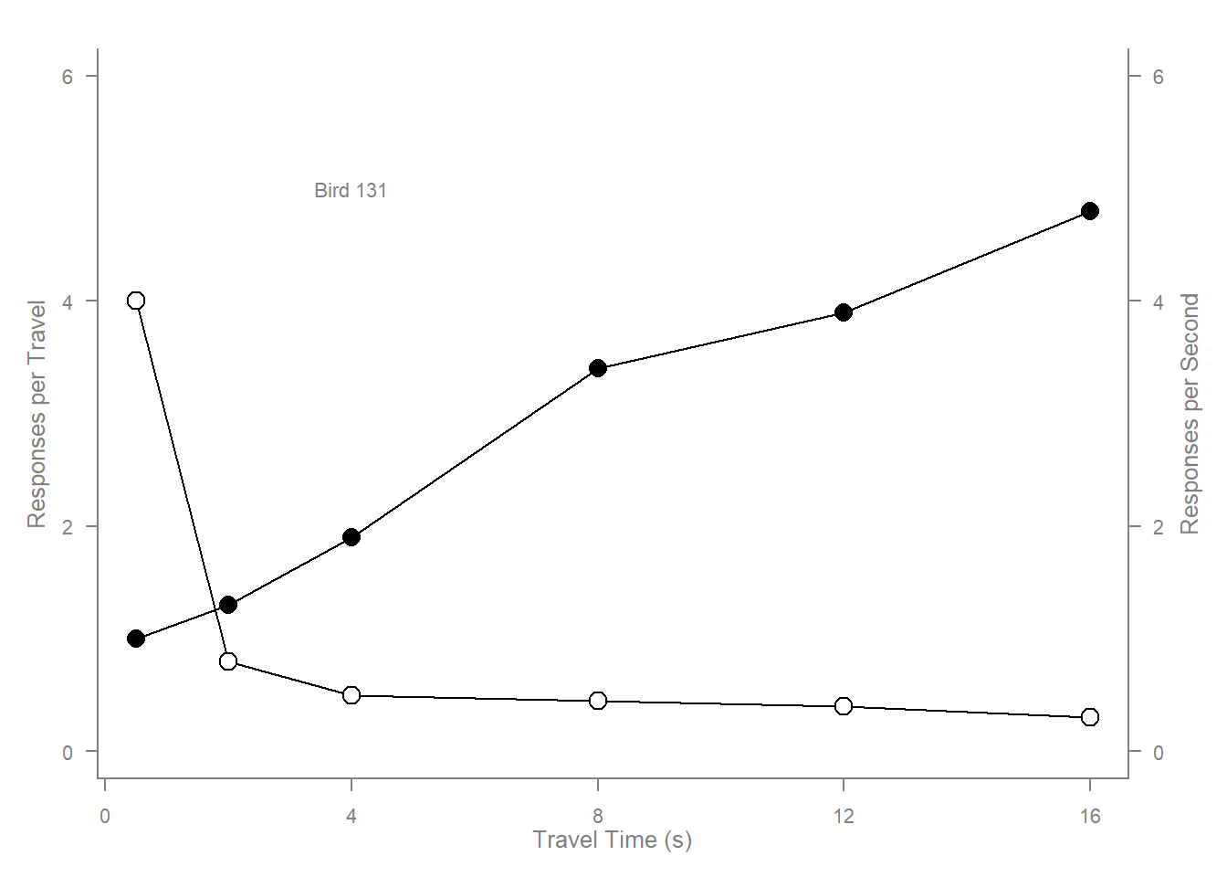
#vector for xx <-c(0.5, 2, 4, 8, 12, 16)#vector for yy1 <-c(1, 1.3, 1.9, 3.4, 3.9, 4.8)#vector for y2y2 <-c(4, .8, .5, .45, .4, .3)# Setting label orientation, margins (4,4,2,4) & text sizepar(las=1, mar=c(4, 4, 2, 4), cex=.7) plot.new() #start a new plotplot.window(range(x), c(0, 6)) #set the x and y range for the plot windowlines(x, y1) #add a linelines(x, y2) #add a linepoints(x, y1, pch=16, cex=2) #add points along the line of type 16 size 2 points(x, y2, pch=21, bg="white", cex=2)#add white points along the line of type 21 size 2 par(col="gray50", fg="gray50", col.axis="gray50") #set the colors of the axes and labelsaxis(1, at=seq(0, 16, 4)) #for the bottom axis set marks to 16 at intervals of 4axis(2, at=seq(0, 6, 2)) #for the left axis set marks to 6 at intervals of 2axis(4, at=seq(0, 6, 2)) #for the right axis set marks to 6 at intervals of 2box(bty="u") #set the box shapemtext("Travel Time (s)", side=1, line=2, cex=0.8) #bottom text, line 2, size .8mtext("Responses per Travel", side=2, line=2, las=0, cex=0.8) #left text, angle 0, line 2, size .8mtext("Responses per Second", side=4, line=2, las=0, cex=0.8) #right text, angle 0, line 2, size .8text(4, 5, "Bird 131") #place text at x=4 & y=5
Rerun anscombe01
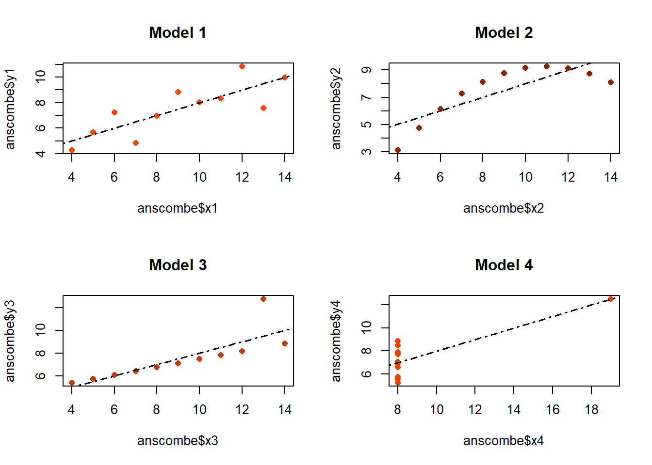
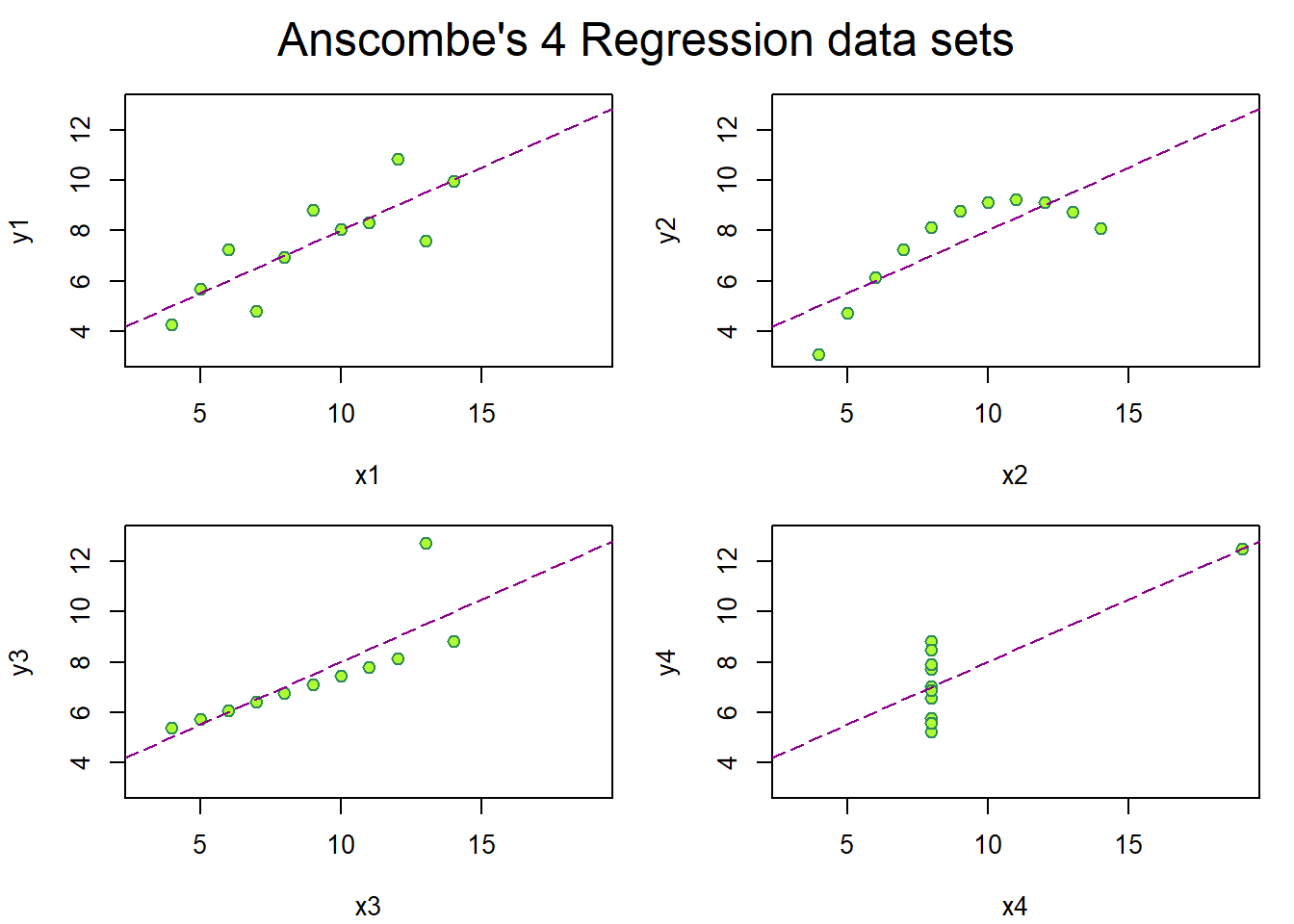
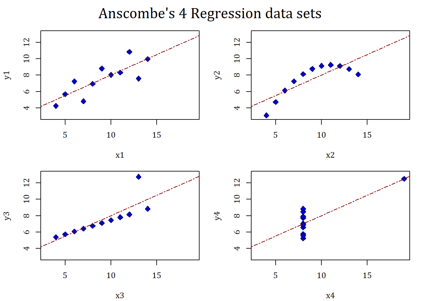
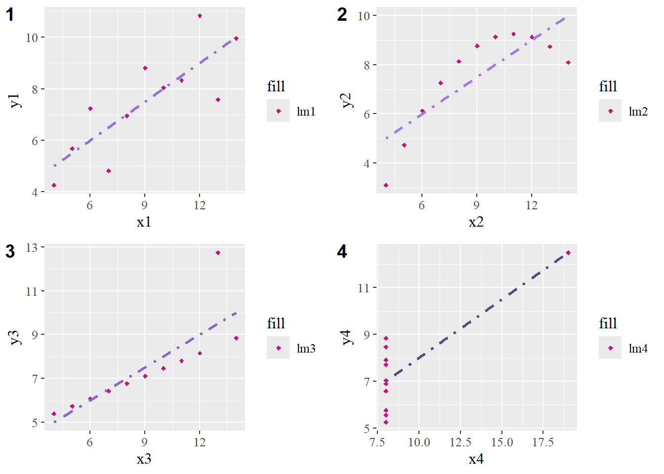
## Data Visualization## Objective: Identify data or model problems using visualization## Anscombe (1973) Quartletdata(anscombe) # Load Anscombe's data#View(anscombe) # View the datasummary(anscombe)
       x1             x2             x3             x4           y1
 Min.   : 4.0   Min.   : 4.0   Min.   : 4.0   Min.   : 8   Min.   : 4.260
 1st Qu.: 6.5   1st Qu.: 6.5   1st Qu.: 6.5   1st Qu.: 8   1st Qu.: 6.315
 Median : 9.0   Median : 9.0   Median : 9.0   Median : 8   Median : 7.580
 Mean   : 9.0   Mean   : 9.0   Mean   : 9.0   Mean   : 9   Mean   : 7.501
 3rd Qu.:11.5   3rd Qu.:11.5   3rd Qu.:11.5   3rd Qu.: 8   3rd Qu.: 8.570
 Max.   :14.0   Max.   :14.0   Max.   :14.0   Max.   :19   Max.   :10.840
       y2              y3              y4
 Min.   :3.100   Min.   : 5.39   Min.   : 5.250
 1st Qu.:6.695   1st Qu.: 6.25   1st Qu.: 6.170
 Median :8.140   Median : 7.11   Median : 7.040
 Mean   :7.501   Mean   : 7.50   Mean   : 7.501
 3rd Qu.:8.950   3rd Qu.: 7.98   3rd Qu.: 8.190
 Max.   :9.260   Max.   :12.74   Max.   :12.500
# Create four model objectslm1 <-lm(y1 ~ x1, data=anscombe)summary(lm1)
Call:
lm(formula = y1 ~ x1, data = anscombe)

Residuals:
     Min       1Q   Median       3Q      Max
-1.92127 -0.45577 -0.04136  0.70941  1.83882

Coefficients:
            Estimate Std. Error t value Pr(>|t|)
(Intercept)   3.0001     1.1247   2.667  0.02573 *
x1            0.5001     0.1179   4.241  0.00217 **
---
Signif. codes:  0 '***' 0.001 '**' 0.01 '*' 0.05 '.' 0.1 ' ' 1

Residual standard error: 1.237 on 9 degrees of freedom
Multiple R-squared:  0.6665,    Adjusted R-squared:  0.6295
F-statistic: 17.99 on 1 and 9 DF,  p-value: 0.00217
lm2 <-lm(y2 ~ x2, data=anscombe)summary(lm2)
Call:
lm(formula = y2 ~ x2, data = anscombe)

Residuals:
    Min      1Q  Median      3Q     Max
-1.9009 -0.7609  0.1291  0.9491  1.2691

Coefficients:
            Estimate Std. Error t value Pr(>|t|)
(Intercept)    3.001      1.125   2.667  0.02576 *
x2             0.500      0.118   4.239  0.00218 **
---
Signif. codes:  0 '***' 0.001 '**' 0.01 '*' 0.05 '.' 0.1 ' ' 1

Residual standard error: 1.237 on 9 degrees of freedom
Multiple R-squared:  0.6662,    Adjusted R-squared:  0.6292
F-statistic: 17.97 on 1 and 9 DF,  p-value: 0.002179
lm3 <-lm(y3 ~ x3, data=anscombe)summary(lm3)
Call:
lm(formula = y3 ~ x3, data = anscombe)

Residuals:
    Min      1Q  Median      3Q     Max
-1.1586 -0.6146 -0.2303  0.1540  3.2411

Coefficients:
            Estimate Std. Error t value Pr(>|t|)
(Intercept)   3.0025     1.1245   2.670  0.02562 *
x3            0.4997     0.1179   4.239  0.00218 **
---
Signif. codes:  0 '***' 0.001 '**' 0.01 '*' 0.05 '.' 0.1 ' ' 1

Residual standard error: 1.236 on 9 degrees of freedom
Multiple R-squared:  0.6663,    Adjusted R-squared:  0.6292
F-statistic: 17.97 on 1 and 9 DF,  p-value: 0.002176
lm4 <-lm(y4 ~ x4, data=anscombe)summary(lm4)
Call:
lm(formula = y4 ~ x4, data = anscombe)

Residuals:
   Min     1Q Median     3Q    Max
-1.751 -0.831  0.000  0.809  1.839

Coefficients:
            Estimate Std. Error t value Pr(>|t|)
(Intercept)   3.0017     1.1239   2.671  0.02559 *
x4            0.4999     0.1178   4.243  0.00216 **
---
Signif. codes:  0 '***' 0.001 '**' 0.01 '*' 0.05 '.' 0.1 ' ' 1

Residual standard error: 1.236 on 9 degrees of freedom
Multiple R-squared:  0.6667,    Adjusted R-squared:  0.6297
F-statistic:    18 on 1 and 9 DF,  p-value: 0.002165
anova(lm1, lm2)
Warning in anova.lmlist(object, ...): models with response '"y2"' removed
because response differs from model 1
Analysis of Variance Table

Response: y1
          Df Sum Sq Mean Sq F value  Pr(>F)
x1         1 27.510 27.5100   17.99 0.00217 **
Residuals  9 13.763  1.5292
---
Signif. codes:  0 '***' 0.001 '**' 0.01 '*' 0.05 '.' 0.1 ' ' 1
anova(lm1, lm3)
Warning in anova.lmlist(object, ...): models with response '"y3"' removed
because response differs from model 1
Analysis of Variance Table

Response: y1
          Df Sum Sq Mean Sq F value  Pr(>F)
x1         1 27.510 27.5100   17.99 0.00217 **
Residuals  9 13.763  1.5292
---
Signif. codes:  0 '***' 0.001 '**' 0.01 '*' 0.05 '.' 0.1 ' ' 1
anova(lm1, lm4)
Warning in anova.lmlist(object, ...): models with response '"y4"' removed
because response differs from model 1
Analysis of Variance Table

Response: y1
          Df Sum Sq Mean Sq F value  Pr(>F)
x1         1 27.510 27.5100   17.99 0.00217 **
Residuals  9 13.763  1.5292
---
Signif. codes:  0 '***' 0.001 '**' 0.01 '*' 0.05 '.' 0.1 ' ' 1
anova(lm2, lm3)
Warning in anova.lmlist(object, ...): models with response '"y3"' removed
because response differs from model 1
Analysis of Variance Table

Response: y2
          Df Sum Sq Mean Sq F value   Pr(>F)
x2         1 27.500 27.5000  17.966 0.002179 **
Residuals  9 13.776  1.5307
---
Signif. codes:  0 '***' 0.001 '**' 0.01 '*' 0.05 '.' 0.1 ' ' 1
anova(lm2, lm4)
Warning in anova.lmlist(object, ...): models with response '"y4"' removed
because response differs from model 1
Analysis of Variance Table

Response: y2
          Df Sum Sq Mean Sq F value   Pr(>F)
x2         1 27.500 27.5000  17.966 0.002179 **
Residuals  9 13.776  1.5307
---
Signif. codes:  0 '***' 0.001 '**' 0.01 '*' 0.05 '.' 0.1 ' ' 1
anova(lm3, lm4)
Warning in anova.lmlist(object, ...): models with response '"y4"' removed
because response differs from model 1
Analysis of Variance Table

Response: y3
          Df Sum Sq Mean Sq F value   Pr(>F)
x3         1 27.470 27.4700  17.972 0.002176 **
Residuals  9 13.756  1.5285
---
Signif. codes:  0 '***' 0.001 '**' 0.01 '*' 0.05 '.' 0.1 ' ' 1
`geom_smooth()` using formula = 'y ~ x'
`geom_smooth()` using formula = 'y ~ x'
`geom_smooth()` using formula = 'y ~ x'
`geom_smooth()` using formula = 'y ~ x'