Assignment 3

Author

Brennan Stout

Published

September 28, 2026

Methods note

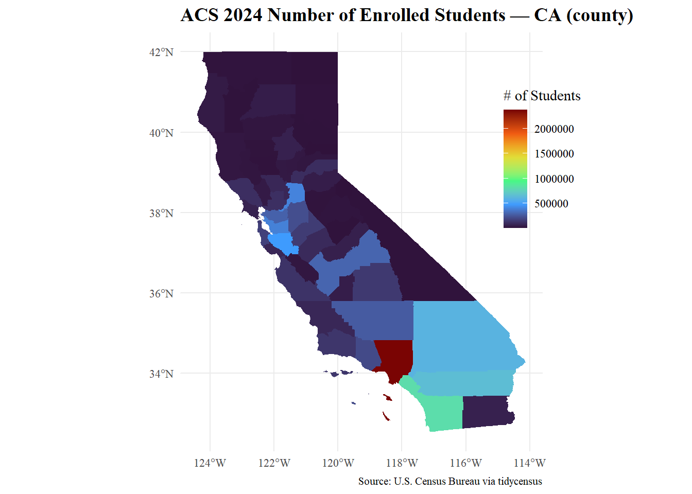
The goal of this was to examine rural urban splits at the county level. Geography: County (State: California) Variables:

Renter occupied housing units
Number of households
Number of enrolled students

A rent rate is calculated as the percentage of households renting. (renter occupied) / (total households) Assumptions: Large percent of renters and a larger number of students in urban counties, showing a younger and more transient population. The margin of error show the uncertainty around the values being mapped. This and the related uncertainty intervals can show if counties are statically different in their rent rates (or not significant if there is an overlap) Interpretation: The map demonstrates the number of students is higher in those urban counties, this is more a reflection of the population density but can also be viewed as the population is younger. Most of the top 10 in rent percent also are major urban counties. (Namely, San Francisco County & Los Angeles)

Warning: package 'tidycensus' was built under R version 4.5.3

Warning: package 'tigris' was built under R version 4.5.2

To enable caching of data, set `options(tigris_use_cache = TRUE)`
in your R script or .Rprofile.

Linking to GEOS 3.13.1, GDAL 3.11.0, PROJ 9.6.0; sf_use_s2() is TRUE


Attaching package: 'dplyr'

The following objects are masked from 'package:stats':

    filter, lag

The following objects are masked from 'package:base':

    intersect, setdiff, setequal, union


Attaching package: 'scales'

The following object is masked from 'package:readr':

    col_factor

Getting data from the 2020-2024 5-year ACS

# 6) Ma
ggplot(acs_wide) + 
  geom_sf(aes(fill = (stu_numE)), color = NA) +
  scale_fill_viridis_c(name = "# of Students", option = "turbo") +
  labs(title = paste0("ACS ", year_acs, " Number of Enrolled Students — ",
                      state_abbr, " (", geo_level, ")"),
       caption = "Source: U.S. Census Bureau via tidycensus") +
  theme_minimal() +
  theme(text = element_text(family = "serif"), # drop if not installed
        plot.title = element_text(size = 14, face = "bold"),
        plot.caption = element_text(size = 8),
        legend.position = "inside",
        legend.position.inside = c(1, 0.7))

top10 <- acs_wide |>
  st_drop_geometry() |>
  arrange(desc(rent_rate)) |>
  select(NAME, rent_rate, rent_moe, rentE, rentM) |>
  slice_head(n = 10)
bottom10 <- acs_wide |>
  st_drop_geometry() |>
  arrange(rent_rate) |>
  select(NAME, rent_rate, rent_moe, rentE, rentM) |>
  slice_head(n = 10)

top10

                               NAME rent_rate    rent_moe   rentE rentM
1  San Francisco County, California 0.6179438 0.005482409  224913  2332
2    Los Angeles County, California 0.5410489 0.001901682 1848466  7040
3       Monterey County, California 0.4792549 0.009322399   63496  1278
4  Santa Barbara County, California 0.4763382 0.008804751   71264  1376
5         Merced County, California 0.4599500 0.013431372   39581  1183
6          Kings County, California 0.4581404 0.019167324   20182   865
7           Yolo County, California 0.4570952 0.013220089   35056  1059
8        Alameda County, California 0.4558944 0.004724704  272737  2935
9      San Diego County, California 0.4543243 0.003150885  532140  3919
10   Santa Clara County, California 0.4492374 0.004873903  296206  3317

bottom10

                           NAME rent_rate    rent_moe rentE rentM
1  Calaveras County, California 0.1603840 0.023415074  2957   444
2     Amador County, California 0.1957616 0.027767714  3150   455
3     Alpine County, California 0.2183908 0.094079591    95    44
4      Modoc County, California 0.2255892 0.054304367   737   182
5  El Dorado County, California 0.2276170 0.011068819 17341   862
6     Nevada County, California 0.2454917 0.018753046 10523   823
7     Placer County, California 0.2522950 0.008514034 39851  1360
8   Mariposa County, California 0.2526638 0.037411603  1897   291
9     Plumas County, California 0.2542836 0.041709178  2048   347
10  Tuolumne County, California 0.2608638 0.026744881  5919   619

print(paste0(“County name:”, sac$NAME, “, Rent Percentage:”, round(sac$rent_rate*100,2), “%, MoE:”, round(sac$rent_moe*100,2),“%, Lower Bound:”, round(sac$rent_lower[[1]]*100,2), “%, Upper Bound:”, round(sac$rent_upper[[1]]*100,2),“%”))

print(paste0(“County name:”, tul$NAME, “, Rent Percentage:”, round(tul$rent_rate*100,2), “%, MoE:”, round(tul$rent_moe*100,2),“%, Lower Bound:”, round(tul$rent_lower[[1]]*100,2), “%, Upper Bound:”, round(tul$rent_upper[[1]]*100,2),“%”))

upper <- list()
lower <- list()

for (n in 1:length(acs_wide$rent_moe)) {
  moe <- acs_wide$rent_moe[n]
  pe <- acs_wide$rent_rate[n]
  lower[[length(lower) + 1]] <- pe - moe
  upper[[length(upper) + 1]] <- pe + moe
}

acs_wide$rent_upper <- upper
acs_wide$rent_lower <- lower

sac <- acs_wide[4,]
tul <-  acs_wide[5,]

print(paste0("County name: ", sac$NAME, ", Rent Percentage: ", round(sac$rent_rate*100,2), "%, MoE: ", round(sac$rent_moe*100,2),"%, Lower Bound: ", round(sac$rent_lower[[1]]*100,2), "%, Upper Bound: ", round(sac$rent_upper[[1]]*100,2),"%"))

[1] "County name: Sacramento County, California, Rent Percentage: 40.98%, MoE: 0.64%, Lower Bound: 40.34%, Upper Bound: 41.62%"

print(paste0("County name: ", tul$NAME, ", Rent Percentage: ", round(tul$rent_rate*100,2), "%, MoE: ", round(tul$rent_moe*100,2),"%, Lower Bound: ", round(tul$rent_lower[[1]]*100,2), "%, Upper Bound: ", round(tul$rent_upper[[1]]*100,2),"%"))

[1] "County name: Tulare County, California, Rent Percentage: 41.55%, MoE: 1.13%, Lower Bound: 40.42%, Upper Bound: 42.67%"

Both counties are proximal counties to larger urban centers, though Tulare is about a third the size of Sacramento County. With the overlap in the confidence intervals, they are not significantly different in their percentages of households who rent.